
Introduction
Today we’re going to talk about one of the most interesting topics nowadays, time series analysis and forecasting. Let me explain you through this post how to train a simply and effective model from Skforecast library in Python.
Skforecast is a Python library that tries to ease Scikit-Learn use, add some interesting tools to pre-processing data and make backtesting. For this purpose, you can work with any of the regressor of Scikit-Learn API (LightGBM, XGBoost, CatBoost, …) and adjust with specific parameters. One of the most interesting features that makes Skforecast my favorite library for time series it’s the wide range of functionalities such as feature engineering, model selection, hyperparameter tuning and others that makes it well-suited for time series analysis.
In the last post, we conducted our analysis and checked all the necessary patterns to ensure that our dataset is ready for forecasting. Please check the link below to understand the assumptions before training the model.
Before train our model
Skforecast provides useful tools specifically designed for time series analysis. One of the first decisions you need to make is which Forecaster to use (Forecaster object in skforecast library is a container that give you the essential tools and methos to train your model). When working with time series data, you likely want to forecast the next t periods rather than just the next one, and there are several methods for calculating multi-step forecasts. In this article, we will focus on one of the most common approaches: recursive multi-step forecasting.
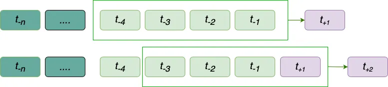
Recursive multi-step forecasting employs a recursive process to predict the next t periods. In this approach, the forecast for each subsequent period are generated sequentially, using the predicted values from previous periods as inputs for future predictions. In this method, lags is the observed/forecasted values that model use to predict the next period, in the example below, we use the last 4 values (lags) to predict the next value.
This method is particularly useful for capturing the temporal dynamics of time series data, as it mirrors how models are often used in real-world scenarios where future values depend on prior outcomes. While error accumulation can be a concern, recursive multi-step forecasting is a strong choice for training models because it allows the model to adapt to the dependencies and patterns within the sequence, ensuring that it learns to handle the compounding nature of sequential predictions effectively.
Model Selection
Once we have our method to capture the trend, we will choose the model to forecast the next t periods. At this point, skforecast allow us to perform any model from scikit-learn API so the amount of chances is bigger than any other library of ML.
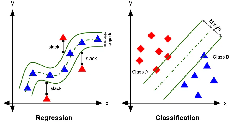
For this example, we will use SVR to train our dataset. Support Vector Regression (SVR) is an extension of Support Vector Machines (SVM), a machine learning technique originally designed for classification tasks. While SVM separates data into classes using a hyperplane, SVR adapts this idea for regression by finding the best fit-line (or curve) within a defined margin of tolerance. Instead of focusing on class boundaries, SVR minimizes errors by considering only points outside the margin, called support vectors.
SVR allows you to use a wide range of hyperparameters, the purpose of this article is not to explore the meaning of each one, let’s assume you are already familiar with them.
Data Split
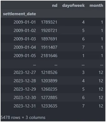
To prepare our dataset in train-test subsets, we begin by mapping the days of the week to numerical values, transforming the textual day names into a numeric format to use as an exogenous variable. The dataset, already a time series, is resampled to ensure a daily frequency, and only the relevant columns (nd, dayofweek, and month) are retained to streamline further analysis.
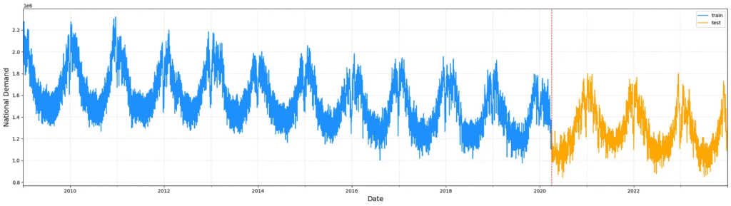
Once processed, the dataset is split into training and testing subsets. A 25% portion of the most recent entries is designated for testing, while the earlier 75% is reserved for training. This approach maintains the temporal order of the data, ensuring that the test set reflects future points relative to the training data, crucial for accurate time-series model evaluation.
Training and Validation
A brief explanation of how easy it is to structure your model using this library. Naturally, you can expand this schema with multiple objects to enhance the accuracy of your model. However, even with this easy schema, you’ll likely achieve satisfactory results.
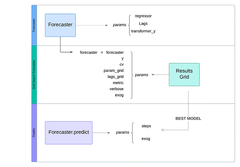
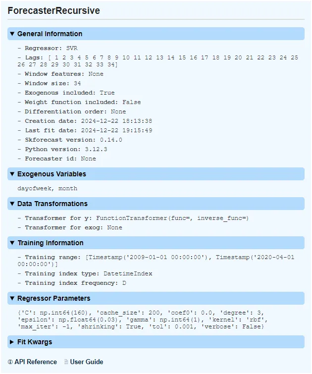
At first time, we set the forecast object, using RecursiveForecast from skforecast library
forecaster = ForecasterRecursive(
                regressor = SVR(kernel='rbf', epsilon=0.05, gamma=1, C=100),
                lags=90, #trying to train with last 3 months lag / 90 days
                transformer_y = FunctionTransformer(func=np.log, inverse_func=np.exp)
)
At this use of case, our instance contains the next params:
- Regressor: An instance of a regressor compatible with the scikit-learn API. The hyperparameters we will set (kernel, epsilon, gamma and C) is not important at this point, so you can set standard values.
- Lags: Periods used as predictors.
- Transformer_y: In most situations, you’ll need to scale your dataset. In this example, we aim to forecast the national demand electricity and the difference between values is too large to capture the trend effectively. We use a logarithmic transformation to train our model and the inverse transformation to plot the results.
Now, it’s time to set up our hyperparameters.
At this point, you have two options. Manually set and test for each combination, evaluate all the results and compare them using metrics or you can use the grid_search_forecaster function.
This tool is very useful to test and set the best parameters, you simply need to understand your dataset and define a dictionary with the parameters that the model has to explore.
results_grid = grid_search_forecaster (
    forecaster = forecaster,
    y          = df_train['nd'],
    cv         = fold,
    param_grid = params,
    lags_grid  = lags_overwritted,
    metric     = 'mean_squared_error',
    verbose    = False,
    exog       = df_train[['dayofweek',"month"]]
)
we’re going to explain each param:
- forecaster: Our forecaster object, defined previously.
- y : Values that model will use to train.
- cv : Class to define the rules for splitting data into train and test subsets
- param_grid: Dictionary that contains the parameters as key and lists of choices as values. Our model train this param grid.
params = {
    'epsilon' : np.arange(0.01, 0.3, 0.02),
    'gamma'   : np.arange(1,3),
    'C'       : np.arange(20,200,20)
}- lags_grid: Also you can train your model in differents lags, this option is useful when you are not sure that your model capture seasonality correctly.
lags_overwritted = {str(lag): int(lag) for lag in np.arange(30,120,1)}- metric: Metric to evaluate the model’s goodness of fit.
- exog: Exogenous variables like predictors. At this case, our model increase accuracy using weekdays and months.
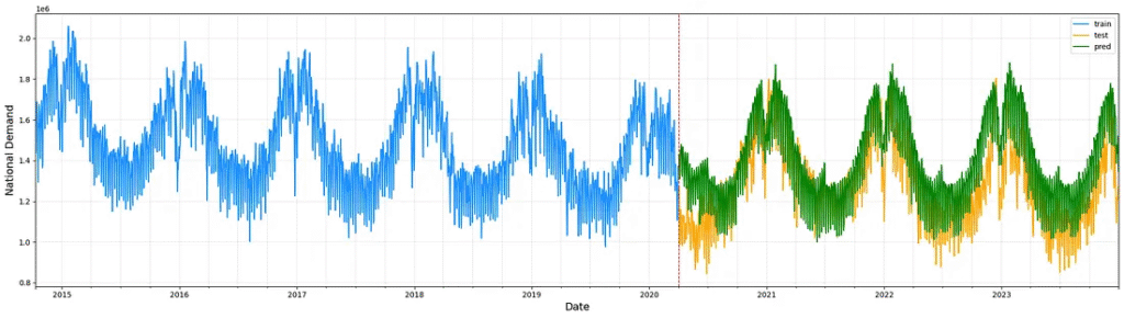
When evaluation comes to an end, we will have two objects: Forecaster with the best fit model and results dataframe.
Your model is ready to predict the next t periods, you only have to use predict method on forecaster object and plot the results.
predictions = forecaster.predict(
                                 steps=steps,
                                 exog=df_test[['dayofweek',"month"]]
)
Conclusions
Skforecast is a powerful library to simplify the training of your model, offering tools to streamline hyperparameter tuning, data splitting, and performance evaluation. Its user-friendly approach allows you to focus on understanding your dataset and refining your predictions, rather than being bogged down by complex coding tasks.
The aim of this article is not to explore all the tools like backtesting or other forecaster objects. The aim is to explain how easy it could be set up and train your model to forecast your dataset.
Perhaps in future articles we will be able to address other functionalities in more depth.
References
Amat Rodrigo, J., & Escobar Ortiz, J. (2024). skforecast (Version 0.14.0) [Computer software]. https://doi.org/10.5281/zenodo.8382788